
Before I became a contractor, parking was tough but doable. I would drive into a parking lot or garage, search for a space for 10 minutes, then quickly rush to my destination. Nowadays, I’m not so lucky. Parking options are restricted, and I’m forced to sometimes rough it up to a half a mile just to go to work. A couple of days ago, I saw a car getting towed near my usual parking spot. I thought to myself “that could have been me.” But then I was inspired. Why not find which streets get you towed? The info is all online!

The craziest thing about this is that the government just freely gives away data like this on a daily basis. The file I found was on “Arlington County Trespass Tows”. I went ahead and downloaded the csv to work offline, but obviously this could have been automated using their JSON feed too. So I began my adventure in R:
# import the tow data
df <- read.csv("tow.csv")  # import the csv
head(df)  # show me the first few records
Results:
                  Date         Company         Location
1  1/1/2018 1:25:17 AM       A1 TOWING 3101 COLUMBIA PK
2 1/1/2018 10:05:05 PM ADVANCED TOWING      2525 LEE HW
3 1/1/2018 12:43:12 AM       A1 TOWING   2000 S EADS ST
4 1/1/2018 10:29:24 PM ADVANCED TOWING 901 N POLLARD ST
5 1/1/2018 11:08:44 PM       A1 TOWING  1515 N QUEEN ST
6  1/1/2018 3:07:38 AM       A1 TOWING    575 12TH ST S
The initial data was promising. I had a date-time, a location (all in Arlington, Virginia), and the towing companies. Next task was to inspect the quality of the data. I started with the companies.
# give me a summary of companies
library(dplyr)  # for pivot table summaries
df %>%  # use this value
  group_by(Company) %>%
  summarize(n())  # give me a count of each company name
Results:
# A tibble: 17 × 2
   Company            `n()`
   <chr>              <int>
 1 ""                    20
 2 "A-1 TOWING"        5756
 3 "A1 TOWING"        11127
 4 "ACCURATE TOWING"     30
 5 "ACURATE TOWING"       1
 6 "ADVANCED TOWING"  32252
 7 "ADVNACED TOWING"      1
 8 "AL'S TOWING"       1018
 9 "ALS TOWING"         295
10 "BLAIR'S TOWING"       5
11 "BLAIRS TOWING"       45
12 "DOMINION WRECKER"     3
13 "HENRY TOWI"           1
14 "HENRY'S TOWING"     843
15 "HENRYS TOWING"      332
16 "PETE'S TOWING"      106
17 "PETES TOWING"        73
It wasn’t as messy as I expected, and there are a surprisingly few number of towing companies in Arlington. Time to clean up the dataframe:
# clean up the data
df$Company[df$Company == "A1 TOWING"] <- "A-1 TOWING"
df$Company[df$Company == "ACURATE TOWING"] <- "ACCURATE TOWING"
df$Company[df$Company == "ADVNACED TOWING"] <- "ADVANCED TOWING"
df$Company[df$Company == "ALS TOWING"] <- "AL'S TOWING"
df$Company[df$Company == "BLAIRS TOWING"] <- "BLAIR'S TOWING"
df$Company[df$Company == "HENRY TOWI"] <- "HENRY'S TOWING"
df$Company[df$Company == "HENRYS TOWING"] <- "HENRY'S TOWING"
df$Company[df$Company == "PETES TOWING"] <- "PETE'S TOWING"
# set company as a factor
df$Company <- as.factor(df$Company)  # sets as factoring

# parse the timestamp so we can pull date information out of it
library(readr)  # for "parse_datetime"
df$Date <- parse_datetime(df$Date, "%m/%d/%Y %I:%M:%S %p")  #sets as date

# get rid of the junk data.  You level of effort should always match that of the data entry representative
df <- filter(df, Company != "")

# Verify the cleanup
df %>%
  group_by(Company) %>%
  summarize(n())
Result:
# A tibble: 8 × 2
  Company          `n()`
  <fct>            <int>
1 A-1 TOWING       16883
2 ACCURATE TOWING     31
3 ADVANCED TOWING  32253
4 AL'S TOWING       1313
5 BLAIR'S TOWING      50
6 DOMINION WRECKER     3
7 HENRY'S TOWING    1176
8 PETE'S TOWING      179
Much better! Next, let’s create some new data features. I want to be able to deconstruct every aspect of time during my analysis:
# Let's define the order of weekdays and months for factorial purposes
DotW <- c("Monday","Tuesday","Wednesday","Thursday","Friday","Saturday","Sunday")
MotY <- c("January","February","March","April","May","June","July","August","September","October","November","December")
# Let's make some new columns in our table
df$Weekday <- weekdays(as.Date(df$Date))  # convert dates into weekdays, adds as column
df$Weekday <- factor(df$Weekday, levels= DotW)  # set factorial numbers based on our list
df$DotM <- format(df$Date, "%d")  # converts dates into days of the month (1-31), adds as a column
df$DotY <- format(df$Date, "%j")  # converts dates into days of the year (1 - 366), adds as a column
df$Month <- months(as.Date(df$Date)) # converts dates to word month, adds as a column
df$Month <- factor(df$Month, levels= MotY)  # set factorial numbers based on our list
df$Year <- format(df$Date, "%Y")  # converts dates to year, adds as a column
# Let's add the city at the end of each location to make a proper address.
df$Address <- paste0(df$Location, ", Arlington, VA")

# view the handiwork
head(df)
Results:
                 Date         Company         Location Weekday DotM DotY   Month Year
1 2018-01-01 01:25:17      A-1 TOWING 3101 COLUMBIA PK  Monday   01  001 January 2018
2 2018-01-01 22:05:05 ADVANCED TOWING      2525 LEE HW  Monday   01  001 January 2018
3 2018-01-01 00:43:12      A-1 TOWING   2000 S EADS ST  Monday   01  001 January 2018
4 2018-01-01 22:29:24 ADVANCED TOWING 901 N POLLARD ST  Monday   01  001 January 2018
5 2018-01-01 23:08:44      A-1 TOWING  1515 N QUEEN ST  Monday   01  001 January 2018
6 2018-01-01 03:07:38      A-1 TOWING    575 12TH ST S  Monday   01  001 January 2018
                          Address
1 3101 COLUMBIA PK, Arlington, VA
2      2525 LEE HW, Arlington, VA
3   2000 S EADS ST, Arlington, VA
4 901 N POLLARD ST, Arlington, VA
5  1515 N QUEEN ST, Arlington, VA
6    575 12TH ST S, Arlington, VA
We now have nine pretty columns of data that can be used to generate just about anything we need. Time to dive into the analysis!
My first question was “do they tow on certain days of the week?” Time to answer that question:
# Most popular towing days of the week
weekday_top <- df %>%  # start a new pivot
  group_by(Weekday) %>%  # group these items by weekday
  summarize(Count = n())  # count all the instances
weekday_top  # Print out the result
Result:
# A tibble: 7 × 2
  Weekday   Count
  <fct>     <int>
1 Monday     5630
2 Tuesday    6077
3 Wednesday  6766
4 Thursday   7266
5 Friday     8539
6 Saturday   9898
7 Sunday     7712
Looks like the tow trucks should not be trusted from Thursday to Sunday.
Next, let’s see if there are certain days of the year that they like to tow.
# Most popular towing days of the year
DotY_top <- df %>%
  group_by(DotY) %>%
  summarize(Count = n())
DotY_top[rev(order(DotY_top$Count)), ]
Result:
# A tibble: 366 × 2
   DotY  Count
   <chr> <int>
 1 315     207
 2 230     206
 3 062     206
 4 259     202
 5 202     200
 6 280     199
 7 212     198
 8 336     192
 9 266     191
10 208     188
# … with 356 more rows
This doesn’t really tell me much. Let’s try a graph:
# Graphed.
library(ggplot2)  # for plots
DotY_plot <- ggplot(DotY_top, aes(x = seq(along.with=DotY), y = Count))
DotY_plot <- DotY_plot + geom_point() + geom_smooth(method = "lm", se=TRUE, formula = y ~ poly(x, 10, raw=TRUE))
DotY_plot <- DotY_plot + labs(title = "Count of Towings by Day of the Year", x = "Day of the Year", caption = "*using method of Loess and the formula 'y ~ poly10'")
DotY_plot
Result:
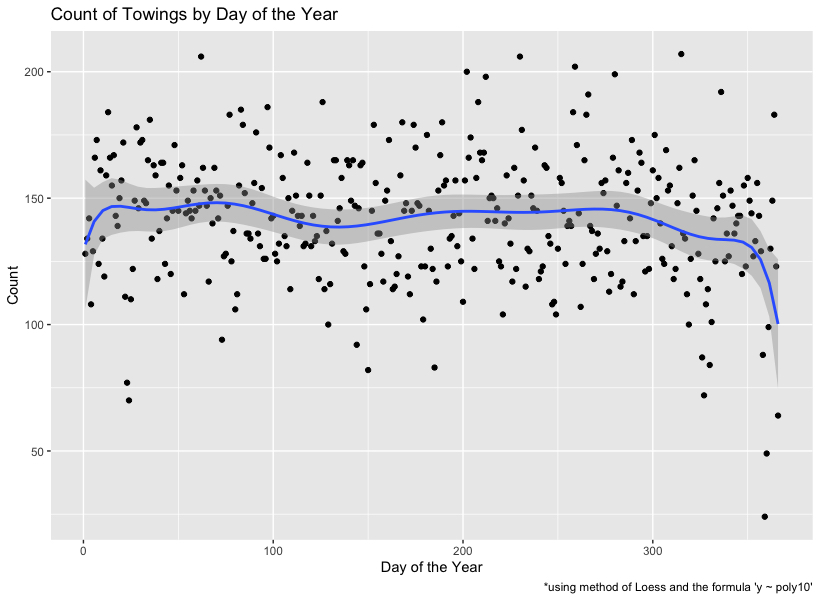
The weirdest thing about this is that they seem to ticket very little during the New Year. Sounds like tow truck drivers are spending time with their families too. Just another reason not to drive drunk during the holidays, folks! What about towing by month?
# Tows by month of the year
month_top <- df %>%
  group_by(Month) %>%
  summarize(Count = n())
month_top <- month_top[order(month_top$Month), ]
View(month_top)
Result:
# A tibble: 12 × 2
   Month     Count
   <fct>     <int>
 1 January    4418
 2 February   4191
 3 March      4540
 4 April      4339
 5 May        4256
 6 June       4256
 7 July       4620
 8 August     4411
 9 September  4298
10 October    4496
11 November   3911
12 December   4152
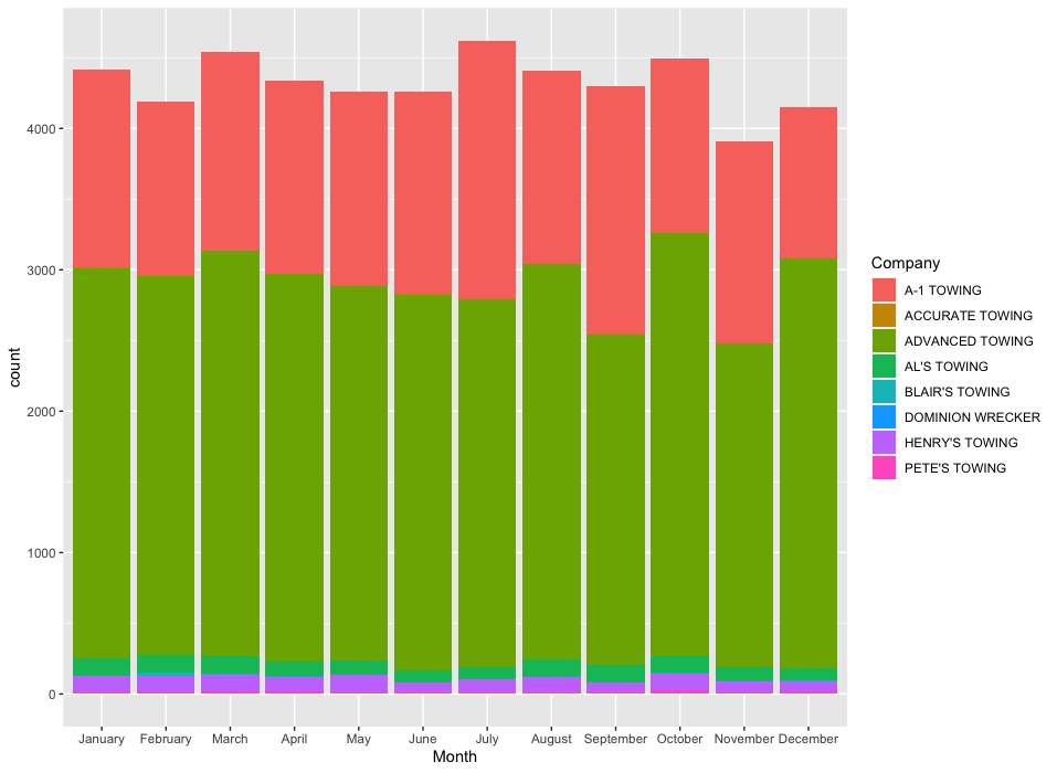
Interesting… Looks like November is a bit of a lull too… Let’s graph it.
# Graphed.  Not proud of the result, but here it is.
date_line <- ggplot(df, aes(x=Month, fill=Company))
date_line + geom_bar()
Result:
As always, what’s the point of even showing data if you aren’t going to plot it on a geographical heatmap. I’m not a huge fan of the process anymore, especially since Google makes you pay for each time you access their geocode API now. I bit the bullet and threw together some credentials and smashed together some ugly code:
if (!requireNamespace("devtools")) install.packages("devtools")
devtools::install_github("dkahle/ggmap")
library(ggmap)  # for google maps plotting
library(dplyr)  # for pivot table summaries

# the pesky API key...
register_google(key = "NeverWillIEverShareIt")

# Heatmap for tows
addresses <- df %>%
  group_by(Address) %>%  # gives me a clean list of non-duplicate addresses
  summarize(Count = n()) # no one cares about this number, but it does make the table compact
addresses$coord <- geocode(addresses$Address) # ONLY RUN THE BELOW ONCE.  TAKES 1 HOUR.
write.csv(addresses, "tow_addresses.csv")  # ESSENTIAL, otherwise you'll be waiting multiple hours
head(addresses)
Result:
  X                             Address Count coord.lon coord.lat
1 1  1 N GEORGE MASON DR, Arlington, VA     1 -77.10048  38.85840
2 2  1 S GEORGE MASON DR, Arlington, VA    17 -77.10648  38.86843
3 3 10 S GEORGE MASON DR, Arlington, VA     1 -77.10695  38.86880
4 4       100 N GLEBE RD, Arlington, VA     2 -77.10230  38.87171
5 5       100 N WAYNE ST, Arlington, VA     4 -77.08537  38.87696
6 6   1000 N RANDOLPH ST, Arlington, VA     1 -77.10980  38.88278
Next, we want to stop working from Google and start working locally on our dataframe. Here’s my approach:
addresses <- read.csv("tow_addresses.csv")

addresses <- addresses %>%
  filter(
  -77.2 <= coord.lon & coord.lon <= -70, # trimmed down to omit Ireland???
  38.83 <= coord.lat & coord.lat <= 40,  # trimmed down to shrink the map.
  )
towings = merge(x=df,y=addresses,by="Address",all=TRUE)  # merged the addresses and data frame into one table
head(towings)
Result:
                             Address                Date         Company            Location
1 1 N GEORGE MASON DR, Arlington, VA 2018-02-14 12:22:56 ADVANCED TOWING 1 N GEORGE MASON DR
2 1 S GEORGE MASON DR, Arlington, VA 2017-12-22 20:45:46 ADVANCED TOWING 1 S GEORGE MASON DR
3 1 S GEORGE MASON DR, Arlington, VA 2017-09-04 03:42:58 ADVANCED TOWING 1 S GEORGE MASON DR
4 1 S GEORGE MASON DR, Arlington, VA 2017-12-09 19:54:03 ADVANCED TOWING 1 S GEORGE MASON DR
5 1 S GEORGE MASON DR, Arlington, VA 2018-02-28 12:35:20 ADVANCED TOWING 1 S GEORGE MASON DR
6 1 S GEORGE MASON DR, Arlington, VA 2018-03-01 11:00:00 ADVANCED TOWING 1 S GEORGE MASON DR
    Weekday DotM DotY     Month Year X Count coord.lon coord.lat
1 Wednesday   14  045  February 2018 1     1 -77.10048  38.85840
2    Friday   22  356  December 2017 2    17 -77.10648  38.86843
3    Monday   04  247 September 2017 2    17 -77.10648  38.86843
4  Saturday   09  343  December 2017 2    17 -77.10648  38.86843
5 Wednesday   28  059  February 2018 2    17 -77.10648  38.86843
6  Thursday   01  060     March 2018 2    17 -77.10648  38.86843
It seems to work. We now have Latitude and Longitude, which will allow us to begin plotting our heatmaps. Next, we’ll use some modified scripts I grabbed from our good ol’ buddy David Kahle who is the maintainer for the ggmap module.
# By Hotspots
qmplot(coord.lon, coord.lat, data = towings, geom = "blank", maptype = "toner-background", darken = .5, legend = "bottomleft") +
stat_density_2d(aes(fill = ..level..), geom = "polygon", alpha = .3, color = NA) +
scale_fill_gradient2("Towing", low = "green", mid = "yellow", high = "red", midpoint=1000)
Result:
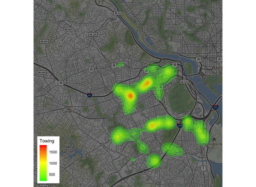
Success! I can clearly see that the street I have been parking on is a verified hotspot for tow trucks. Time to find a new street to park on. Let’s see what else we can do with this data. Patterns of life maybe?
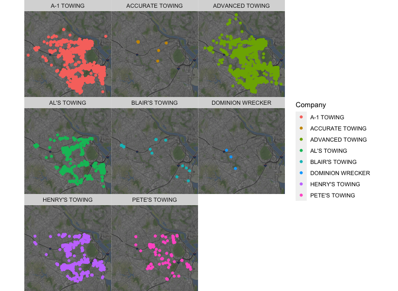
Now let’s see where each of the Towing Companies operate:
# By Company
qmplot(coord.lon, coord.lat, data = filter(towings, Company != ""), maptype = "toner-background", darken = .5, color = Company) +
facet_wrap(~ Company)
Result:
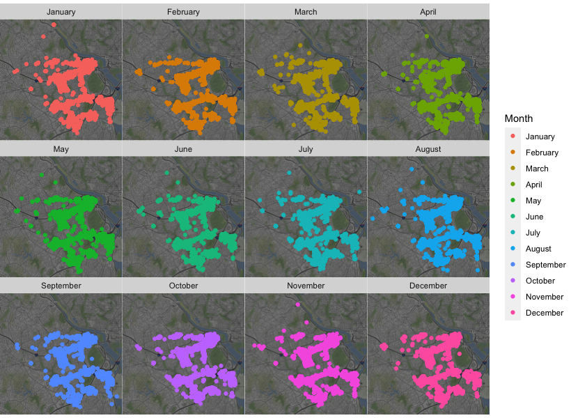
What about by the Month of the year?
# By Month of the Year
qmplot(coord.lon, coord.lat, data = filter(towings, Month != ""), maptype = "toner-background", darken = .5, color = Month) +
facet_wrap(~ Month)
Result:
Would I do this again? Not for free. Is this a great learning experience? Oh yeah! You bet. Here’s the Source Code for my project.
Just go ahead and play around in R-Studio. You’re going to love what you discover about your neighborhood tow trucks.